How to train neural networks for image classification — Part 2
Image classification is a hot topic in data science with the past few years seeing huge improvements in many areas. It has a lot of applications everywhere including SEO. But how is this done?

In part one of this series, I talked about the most basic type of neural networks (dense layer neural networks) and showed how to implement one in Python using Keras (with Tensorflow) to implement a basic image classifier.
In part 2 of this series I will be talking about a slightly more complicated type of neural network architecture using convolutional layers. Convolutional neural networks generally perform better on image processing tasks, and I shall be going into how they work, why they perform better with image classification tasks and how to implement a basic convolutional neural network using Keras.
Layers in a convolutional neural network
As I mentioned in part 1 of this series, there are different types of layers in neural networks with each what effecting a different type of transformation on the data that goes into it.
For image processing there are 2 type of layers that are really important and I shall go into more detail about them here. These are:
- Convolutional layers
- Max Pooling layers
Convolutional layers
In part 1 I showed how to do image processing with a neural network that used dense layers and these are long lines of neurons all connected and we had to flatten the input to a 1-dimensional array before working with it.
With a convolutional layer, the neurons are arranged in 3-dimensions and that means we can feed in our images in the 2-dimensions that represents the data more accurately.
Also, in a convolutional neural network, not all of the neurons are connected as with dense layers. A convolutional layer is modelled on how the visual cortex works in our brains and the ways our brains process what our eyes see.
The way the cells at the back of ours work is that groups of cells with a limited visual field react to light that hits the back of our eyes and all of these bunches of cells with their limited visual fields are all connected to neurons in the brain where they are processed and built up into one big image that we understand.
With a convolutional neural network, we layer we have one neuron per pixel in the image. We also specify the layer’s kernel size which means how many neurons we want to be in these ‘groups’ of neurons that make up the visual fields that make up the image. The outputs from one group of neurons that make up a kernel are connected to one input in the preceding layer.
In this way, the image is processed as the convolutional layer convolves (i.e. moves across) the image processing each group of pixels in and passing the outputs to the preceding layer for processing. This is pretty abstract and can be better visualised by a diagram:

The guys at Deep Lizard do a really good job at explaining this too and I highly recommend you look here for an explanation about how convolutional layers work.
Another important property of convolutional layers are the filters and when we create a convolutional layer we specify how many filters we want it to have. It is the filters that can detect patterns in the image and the filters form layers within each convolutional layer (not between convolutional layers — yes, this does bend your head).
All neurons in a filter share the same weights and each neuron in one filter is connected to its counterpart in the next filter so that the output of one filter is passed to the corresponding set of neurons in the next filter. This gives us a structure which looks something like this:

As I’ve mentioned above, the purpose of each filter is to detect different patterns in the image and as the network is trained it will converge on which patterns within each filter will enable it to recognise each image. The output of each filter is called a feature map and it is these that are used by the network to decompose an image down into its component pieces.
Neurons in a filter evolve specific patterns and fire when they see that pattern and output the result into the next filter. All of these feature maps can then be build up into the final image and can be used to process it. As an example of what this looks like:

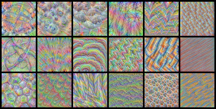
In CNN architectures it is standard to start with fewer filters to detect top-level features in the image and then to increase the number of filters as we get deeper into the network to detect more specialised features. If you need more clarity on this then there is a good video on this topic here. As an aside, the image at the start of this post shows different feature maps for a more complex network.
If you need a more visual way of how these networks work then this video is good and shows how different networks process images in real-time:
Max Pooling Layers
Convolutional layers are usually paired with max-pooling layers and if you understand how convolutional layers work then max-pooling layers are simple.
Their purpose is to sub-sample an image highlighting the most important areas for the network to process. The reason we need these is to reduce computational complexity and to reduce the dimensionality of the image.
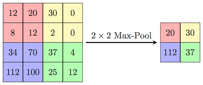
A max-pooling layer isn’t trainable like convolutional layers. All it does is look at all of the pixels in a receptive field, picks the one with the highest value and passes that on to the next layer in the network.
It is really easy to visualise this with a spreadsheet approach and the guys at Deep Lizard have a really good video on this here. A good way to visualise this is as follows:

Solving Fashion NMIST using a CNN in code
The full code to do this is available on my Github page, but I will take you through the highlights below. I will be using a CNN to build a simple classifier for the Fashion MNIST dataset and I will be comparing its performance to the dense layer network I used in part 1.
Using Keras as a part of Tensorflow we can implement the following simple CNN:
model = keras.models.Sequential([keras.layers.Conv2D(64, 7, activation=”relu”, padding= “same”, input_shape=[28, 28, 1]),
 keras.layers.MaxPooling2D(2),
 keras.layers.Conv2D(128, 3, activation=”relu”, padding=”same”),
 keras.layers.Conv2D(128, 3, activation=”relu”, padding=”same”),
 keras.layers.MaxPooling2D(2),
 keras.layers.Conv2D(256, 3, activation=”relu”, padding=”same”),
 keras.layers.Conv2D(256, 3, activation=”relu”, padding=”same”),
 keras.layers.MaxPooling2D(2),
 keras.layers.Flatten(),
 keras.layers.Dense(128, activation=”relu”),
 keras.layers.Dense(64, activation=”relu”),
 keras.layers.Dense(10, activation=”softmax”)
 ])
To explain this code:
- We create a Keras sequential network, which means that this network will be a sequence of layers stacked on top of each other
- The first layer is a convolutional layer with 64 filters and a kernel size of 7 x 7. We use a relu activation function. As this is the first layer in the network, we also specify an input of 28 x 28 (pixels) x 1 (one colour channel only as this is a greyscale image)
- The next layer is a max-pooling layer that sub-samples the data from the previous layers in a 2 x 2 grid
- We then repeat a similar structure where we have 2 convolutional layers with increasing filter numbers to pick up greater feature definitions as we progress further into the network; this is followed by another max-pooling layer to sub-sample the data further
- Finally, we have a sequence of dense payers (after the flatten layer to put the data into a 1-dimensional array that dense networks need); the dense layers become more focused until the final layer has 10 neurons, which is equal to the number of classes in the data set; the final also uses a softmax activation function as it outputs probabilities that an image belongs to a specific class
We can examine the structure of this network by calling the models summary method:
model.summary()Model: "sequential"
_________________________________________________________________
Layer (type) Output Shape Param #
=================================================================
conv2d (Conv2D) (None, 28, 28, 64) 3200
_________________________________________________________________
max_pooling2d (MaxPooling2D) (None, 14, 14, 64) 0
_________________________________________________________________
conv2d_1 (Conv2D) (None, 14, 14, 128) 73856
_________________________________________________________________
conv2d_2 (Conv2D) (None, 14, 14, 128) 147584
_________________________________________________________________
max_pooling2d_1 (MaxPooling2 (None, 7, 7, 128) 0
_________________________________________________________________
conv2d_3 (Conv2D) (None, 7, 7, 256) 295168
_________________________________________________________________
conv2d_4 (Conv2D) (None, 7, 7, 256) 590080
_________________________________________________________________
max_pooling2d_2 (MaxPooling2 (None, 3, 3, 256) 0
_________________________________________________________________
flatten (Flatten) (None, 2304) 0
_________________________________________________________________
dense (Dense) (None, 128) 295040
_________________________________________________________________
dense_1 (Dense) (None, 64) 8256
_________________________________________________________________
dense_2 (Dense) (None, 10) 650
=================================================================
Total params: 1,413,834
Trainable params: 1,413,834
Non-trainable params: 0
As can be seen, this model has a total of 1,400,000 trainable parameters, versus 286,000 trainable parameters for the dense layer network that I used in part 1. This means that CNNs are very computationally intensive and so if you do work with them you are definitely going to need GPU accelleration on your home machine. Or to use Google Colab with a GPU terminal enabled.
If we train the model with 30 epochs and test the model on test dataset we see the following:
model.evaluate(X_test,y_test)313/313 [==============================] - 1s 4ms/step - loss: 0.4174 - accuracy: 0.9054[0.41743409633636475, 0.9053999781608582]
We get an accuracy of 90% versus an accuracy of 88% for a dense layer. While this isn’t state-of-the-art it is a big improvement.
Why do CNNs work so well for image recognition?
The reason why CNNs work so well for image recognition is that as mentioned above the neurons in a filter all share the same weightings. This means that once the filter has learned to recognise a particular shape in an image, it doesn’t matter whereabouts in the image the shape appears the network will recognise it.
This is opposed to a dense layer network which can learn to recognise shapes, but only at specific points in an image and it won’t generalise to anything else. This is why CNNs are so powerful for image recognition.
Thanks for reading
We’ve looked at how a dense layer neural network and a convolutional neural network perform on a very common image processing dataset. I hope you found this useful and if you have any questions feel free to reach out.
